A DISTANT, COMPLEX SUPERNOVA REMNANT G344.7-0.1

Wow, hey guys! It has been quite the hiatus and I do apologize. But, hello!😀 As you can see, I have moved things over to a new web host (WordPress). I lost quite a bit of formatting in many of my old posts so it took me some time to go through and fix it all, though I need to go back (again) to fix how some of the posts appear on mobile devices, so thank you all so much for your patience with me during this time 😇🥰

Me after moving my whole website by myself 😅

I thought it was about time to not only come back here to continue my regular blog posts, but to go ahead and conclude the second paper that I started discussing back in September and is available here.

To briefly remind us what we are dealing with:

We have a known supernova remnant (SNR) located along the Galactic plane with the Galactic coordinates (G) 344.7 (longitude, in degrees), -0.1 (latitude, in degrees). Hence, the identifier “G344.7-0.1”.
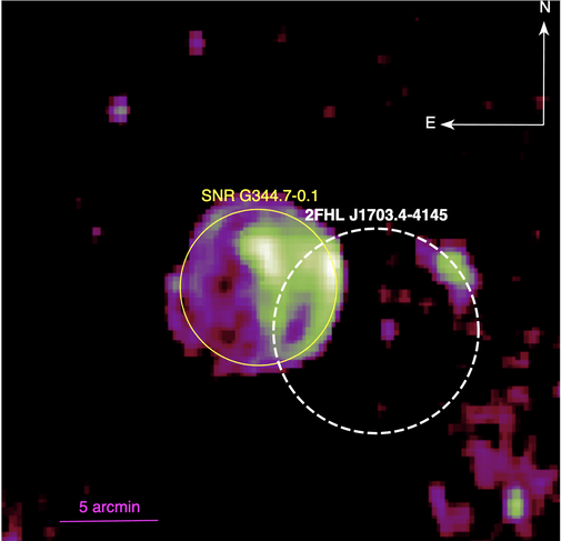
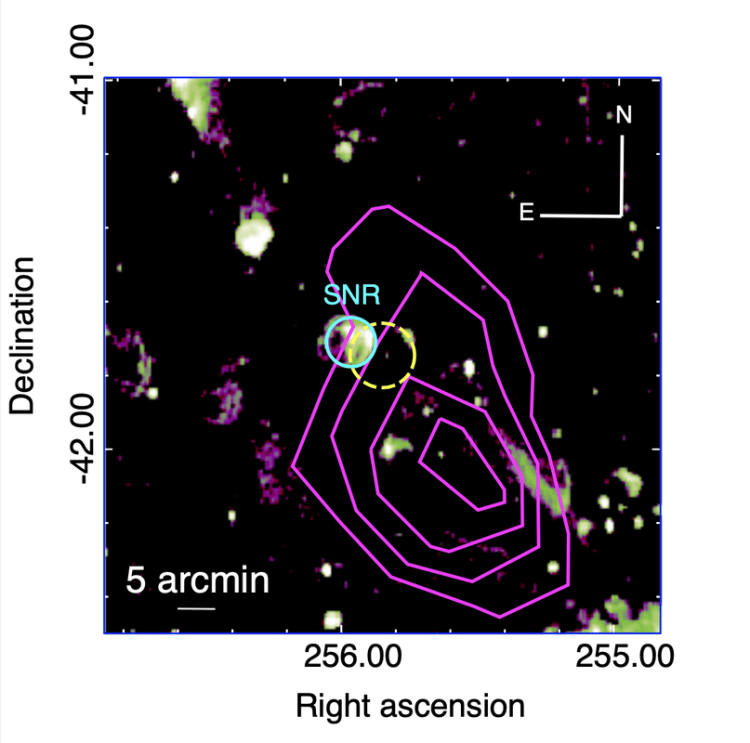
Faint, point-like gamma-ray emission, which is detectable at energies > 10 GeV with the Fermi-LAT, overlaps with the Western edge of the remnant, suggesting some kind of connection.
Extended very high energy emission above 1 TeV is adjacent to the > 10 GeV emission location, suggesting that whatever is responsible for the > 10 GeV gamma-rays is also responsible for the very high energy gamma-rays above 1 TeV.
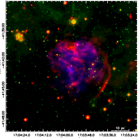
Analyzing old archival X-ray observations from the XMM-Newton X-ray Space Telescope, we discover the SNR is dominated in this energy band by thermal X-rays with no hint of non-thermal emission in or around the SNR.
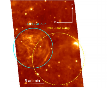
Finally, there is a notable IR filament that overlaps well into the confidence region for the gamma-ray emission (i.e. the region where the gamma-ray emitting source is most likely to be located).

SPITZER 24 μm image of SNR G344.7–0.1 with 2FHL J1703.4–4145 95% uncertainty region indicated. Note the bright filament on the western edge of the SNR that overlaps well into the 2FHL region (From Eagle et al., 2020 😉).

There are a lot of cool things happening here. Because my first source turned out to be a shock-cloud interaction (probably), I was definitely wondering if I was somehow looking at another one! The evidence seemed to line up in a strikingly similar way to the Vela SNR. But G344.7-0.1 is a lot farther away from us than Vela, so that introduces some extra challenges to trying to figure this out.

In fact, Vela is only about 1,000 light years away from us. That means it takes 1,000 years for LIGHT to travel from the pulsar to us, which is roughly 5,879,000,000,000,000 miles from Earth or 9,461,000,000,000,000 kilometers. But really, as far away as that might sound, that’s still relatively close. Look at some similar systems plotted by distance from us (the Sun/Solar system) with respect to the larger Galaxy we belong to, the Milky Way 🥰.

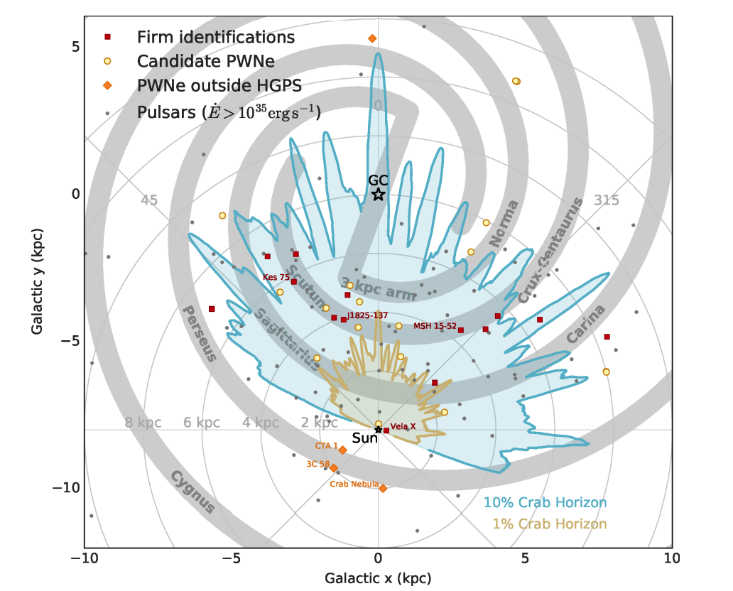
Picture diagram of the Milky Way and its spiral arms, along with some PWNe candidates (remember PWNe = pulsar wind nebulae which is what I study 🤓) marked including the PWN within the Vela SNR, dubbed “Vela-X”. Also indicated are other objects in our Galaxy like really energetic pulsars! Find Vela-X.

The above image is borrowed from an analysis on objects like the Vela SNR in the HESS Galactic Plane Survey released in 2018. The free version of the article can be found here. Look how close Vela-X (a component to the Vela SNR) is to us within our Galaxy!

The black outlined star with the initials “GC” represents the Galactic Center (GC) which is about 8 kiloparseconds away from our Solar system. That’s roughly 26,000 light years away from us. That’s right! That means that the light from the center of our own Galaxy has to travel for 26,000 YEARS before it reaches us! And yes, it’s moving as fast as it can!

Now, this is all relevant to G344.7-0.1 for the following reason: Measuring the distance of a far-away SNR like this one can be tricky, so our estimates leave us with some pretty big margins of error, but we estimate this particular system is at least 3 kiloparseconds away (about 10,000 light years) but could be on the opposite side of the Galaxy anywhere between 9 kiloparseconds (kpc for short) and 14 kiloparseconds (or almost 46,000 light years away from us 😧). The uncertainties attached to these huge ranges in distance haunt us throughout our analysis!

It also haunts us in the quality of data that is available for this source. For Vela, we had so much literature and surveys to sift through, which ultimately gave us the “smoking gun” for the shock-cloud interaction, the hydrogen cloud that shared the same shape and location as the higher energy emission we had discovered! But this source, G344.7-0.1, being much farther away, does not have adequate imaging for those same surveys, so we aren’t able to make any firm conclusions about what the SNR could be running into.

This is because the angular resolution of most available surveys for data covering our SNR region was just not gonna cut it to resolve any meaningful connections. This time, we had to really think about the physics involved here to be able to interpret our findings and offer a consistent explanation.

So what did we do? Our most favorite thing! We took all of the data we could measure for this source in light waves — from radio wavelengths to TeV gamma-rays — and we tried to put it on a plot (remember those spectral energy distributions we discussed some time back?). Then, with some software tools like Python, we can apply relevant physics equations to the processes going on and try to predict what we would observe and then compare that to what we actually see. This way, we control the physics and processes that explain the observations so we can make meaningful conclusions on what the possible scenario is going on here.

The spectral energy distribution (SED) model constrained to 3FHL (lower energy gamma-rays) and HESS (higher energy TeV gamma-rays) data. The solid grey line (hadronic scenario) and the dashed grey line (leptonic scenario) demonstrate the resultant γ-ray spectrum of radiation from relativistic protons or electrons, respectively. Right: IC decay (i.e., leptonic scenario, blue) and pion decay (i.e., hadronic scenario, grey) model contour plot for the spectral fitting results, marking the 1σ and 2σ uncertainties. The black dot shows the best-fit values.

Recall that we had all of the following wavelength ranges on this source: radio, X-ray, Fermi (MeV-GeV) gamma-rays, and HESS TeV gamma-rays. In the plot above, however, you’ll notice that only the gamma-rays are plotted on our spectral energy distribution (SED) plot. This is because these models assume that the particles radiating the observed emission is all one population with the same characteristics — same radiative mechanisms, same interaction processes, same average energies, etc — and this may not always be a good assumption to make. It is entirely possible that the particles responsible for emitting in radio waves are totally separate from the population responsible for the higher energy emission!

As we plotted all of the radio — gamma-ray data, it became clear that there must be more than one particle population present: one to explain the radio and X-ray data and one to explain the higher energy data. However, our model is limited in this regard. If we need to “add” more particle populations to the model, it gets very complicated, and so we are unable to investigate this further. As a result, we limit ourselves to only trying to characterize the population behind the high-energy emission in the gamma-ray regime. Hence, the SED above only plots the gamma-ray data points.

Now, we are almost there for coming up with a way to understand what we are seeing. We now know that the high energy emission is disconnected in a particular way from the lower-energy (radio and X-ray) emission from our supernova remnant. This is interesting since the radio and X-ray emission is confined to the supernova remnant itself: the radio and X-ray emission fill the SNR, but both the radio and X-ray emission steeply decline just beyond the SNR shell. On the other hand, the gamma-ray emission is located on the Western edge of the SNR, with higher-energy gamma-rays extending to the South-East of the SNR shell. This picture seems consistent with the current model results that these are two separate populations.

Based on the X-ray and radio location and properties, we know the SNR has accelerating (i.e., radiating) particles that are emitting synchrotron radiation largely in radio, but these particles are not the same ones generating the gamma-ray emission. We can also tell by the SED above, that we cannot make any distinction with the data alone to say if it’s more likely to be protons (hadronic scenario) or electrons (leptonic scenario) that is responsible for the observed emission… Did we hit a road block? Is this where our journey ends?

The answer is no. We still have some information to consider. We need to consider now both the morphological properties (aka how the SNR looks in each wavelength) and compare it to our best-fit model and the estimated parameters (properties of the particles) to try and understand the most likely origin for the high-energy emission.

This is a lot to digest though, so you know what time it is! 😉 Next time, we will wrap up with the big picture for this object and I’ll also explain a little more about what measurements we can make from our best-fit model (particularly the right panel shown in the above image).

Quiz! Take it here.

And as always, check out the free version of the article being summarized here.

LIGO GRAVITATIONAL WAVE (GW) EVENT GW190521

May 21, 2019, the Laser Interferometer Gravitational-Wave Observatory (or LIGO) detected a signal that came from the merging of two black holes.

Wow! Where to begin. One of the world’s first gravitational wave detectors, LIGO, is a pair of laser interferometers located 3,000 km apart or about 1,800 miles. Locations are the Hanford Observatory in Washington and the Livingston Observatory in Louisiana. This detector is incredibly sensitive, detecting some of the weakest signals known to man. A short video summarizes the first observation made by LIGO told directly by the leading scientists in the endeavor. These scientists, Rainer Weiss, Kip Thorne, and Barry Barish, won the 2017 Nobel Prize in Physics for the discovery. LIGO is supported by the National Science Foundation (NSF), Caltech, and MIT.

How do the interferometers work? The LIGO collaboration provides excellent video and explanation here.

We have come a long way with our understanding of the Universe and general relativity. Gravitational waves (GWs) are detected as disturbances in the interferometer. We can measure the duration and the frequency evolution of the signal and from that, we can apply general relativity theory to understand what took place and where for the GW event to occur. In 2015, LIGO reported the first ever detection of such an event, and it was determined to be from the merging of two black holes. These black holes merged to form an ever larger black hole.

Since then, LIGO and the twin observatory, VIRGO in Italy, have made several more observations of GW events! Isn’t that amazing? Most of the observations are consistent with general relativity (GR) modeling for binary black hole mergers with a single binary neutron star merge event, GW170814. All of these events are unique for different reasons but I will focus on the most recent detection yet, GW190521.

GW190521 is another binary black hole merge event, with the observed measurements being completely consistent with GR numerical simulations where they have assumed a quasi-circular compact binary coalescence – this is basically fancy talk describing two black holes slowly spiraling together in their respective circular orbits until collapsing and merging together. So, they were able to determine the most likely scenario to generate a GW signal with the same properties as GW190521 was a binary black hole system that ended with the two black holes merging together to form an altogether larger black hole.

First of all, this is amazing that this kind of research is possible. I just – wow. I mean, right? This is just incredible. The unimaginable has been imagined and then brought to life! Thank you, Albert Einstein. Second of all, this binary black hole (BBH from now on) merge event is special for two main reasons.
1) The two black holes that merged together have been measured to be 85 and 66 times the mass of the Sun, which we denote using M ☉. The primary black hole (BH), the 85 M ☉ one, is especially intriguing. The current understanding of stellar evolutionary theory for very massive stars predict that no black holes should be formed from stellar collapse between about 55 to 120 M ☉. Of course, there are uncertainties surrounding where exactly this mass “gap” really lies but, the physics and modeling all appear to predict the same thing — no black hole remnants should be formed from stars between 55-120 M ☉, give or take. But how much give or take? In the second report characterizing the astrophysical properties of GW190521, they report that the probability one of the black holes that merged together has a mass within the mass gap is 99%.
2) The mass of the final BH from the merge event is estimated to be ~150 M ☉. This is the first strong evidence for the existence of an intermediate black hole. An intermediate black hole is a black hole that ranges in size from ~100s to ~100,000s the times the mass of the Sun. LIGO has detected several BH merge events, but only from stellar-mass black hole systems so far. GW190521 is the most massive BBH merge event observed to date!

Illustration showing the masses of the two black holes that formed the intermediate black hole. How did the two black holes form before merging? [Image credit: LIGO/Caltech/MIT/R. Hurt (IPAC).]

The LIGO community announced the detection only just Sept. 2, 2020. Below is the GW detection signal from both LIGO detectors and VIRGO, and the signal represented in the time-frequency domain in the images displayed in the bottom panels. The signal was very short, with a duration of only 0.1 seconds and ranged in frequency from 30-80 Hz.

The GW event GW190521 observed by the LIGO Hanford (left), LIGO Livingston (middle), and Virgo (right) detectors. Times are shown relative to May 21, 2019 at 03:02:29 UTC. s. The bottom row displays the time-frequency representation of the whitened data using the Q transform. From Abbott + 2020

I believe it was first reported in Physical Review Letters here, of which the above image is adapted from. A really cool short video is shared below that nicely reiterates what I’ve just mentioned (and then some!).

Other cool materials are available here: https://www.ligo.org/detections/GW190521.php including a video of a numerical simulation of a binary coalescence that reproduces GW190521 (which I also display directly below because its COOL).

Above: Numerical simulation of two black holes that inspiral and merge, emitting gravitational waves. The black holes have large and nearly equal masses, with one only 3% more massive than the other. The simulated gravitational wave signal is consistent with the observation made by the LIGO and Virgo gravitational wave detectors on May 21st, 2019 (GW190521).

A New Frontier: Gravitational Wave Astronomy

Einstein predicted in general relativity theory that changes in the gravitational field will travel through the universe at the speed of light. These are gravitational waves and were only first confirmed in 2015. In 2020, we discover the most massive black hole merge event observed to date, and it happens to be pushing the limits of what we understand about the evolution of massive stars and, the nature and formation of intermediate sized black holes. Today, there are currently no confirmed intermediate black holes (IMBHs). There are several candidates, most of which reside in dwarf galaxies and are associated to low-luminous active Galactic centers. However, having no firmly identified IMBHs leaves many questions unanswered. How do IMBHs form? What conditions are necessary? The final BH responsible for GW190521 may give us clues and perhaps, future detections by LIGO and VIRGO may further reveal the Universe’s secrets.

I’ve been reading into this some and will discuss a short letter that investigates the origin of the primary 85 M ☉ BH of GW190521 in the coming blog post!

PAPER II: (ANOTHER) NEW GAMMA-RAY SNR

This particular object I began looking more into right around the time I was also preparing for the written qualification exams at Clemson University. PHEW that is a stressful time to look back on. Maybe I’ll write more about the PhD process in the program in another blog post but, for now, let’s focus on the second Fermi object I investigated. I had a task to gather data for 12 newly detected very high energy sources – or VHE, which we will define at an energy E > 50 GeV which is among the highest energy for light, the gamma-ray range. The gamma-ray space telescope, Fermi, had just discovered these sources and were reported in 2016 (free and public pdf version available here). I was looking at multiple sources at once but, one particular source, led me somewhat down a rabbit hole and led to my second paper (in review but hopefully close to acceptance and publishing!) on the multi-wavelength analysis of the supernova remnant, G3447.1-0.1, which is found to be a likely origin for the newly discovered gamma-ray emission at the edge of the remnant. Does this sound familiar? It should! My first report was also on the discovery of gamma-ray emission on the edge of the Vela supernova remnant (SNR). Coincidence? Yes. Lol. Though this time the physics was a little more complicated but, all the more exciting!

First thing I noticed was this new gamma-ray source was pointing to the SNR G344.7-0.1, pictured below.

Radio (843MHz), the SNR is indicated and the 95% confidence region of the gamma-ray source is the white dashed circle.

The SNR as seen in 3 different wavelengths of light. In blue is soft X-ray emission (soft meaning low energy), and red and green represents 24 and 8 um infrared emission.

The same X-ray emission seen in the middle panel is shown in the color image here. The black lines are showing you the flux contours of the radio image from the left panel

Admittedly my only experience so far with gamma-ray objects was the emission we identified as a shock-cloud interaction on the west edge of the Vela SNR and, so far, I was looking at another SNR with gamma-ray emission appearing on the west edge which overlapped with bright radio emission and a strong infrared filament. The bright radio emission can be seen in the left panel above. The green color is showing you where the radio emission brightens which is seen to be on the north and western regions. Similarly, we see brighten infrared emission in the northern-central and western regions as shown in the middle panel. Do you see the red filament in the middle panel? This coincides with the gamma-ray position and bright radio emission. Interesting.

By the way, the above images can be found in the following reports: (left) Eagle et al., 2020 (arXiv pdf version here), (middle) Combi et al., 2010 (arXiv pdf version here), and (right) available here.

So what does this mean, exactly? Well, in general, where one might see increased emission accompanying high energy emission, like this gamma-ray source, points to some kind of interaction that would accelerate these particles to radiate at the varying wavelengths. Each wavelength provides us different information about the particles responsible for the radiation and how they must be interacting with their environment. This also means we can infer what that environment is made up of.

Recall my first report we were able to determine the presence of a small neutral hydrogen cloud that was found to coincide precisely with the western wall of the Vela SNR that paired with the observed gamma-ray emission there. We can plausibly describe the gamma-ray emission as arising between the remnant’s forward shock – that is, it’s outer layer that was blast into the interstellar medium first at the time of explosion – is running into its surroundings and is colliding with and disturbing the material.

Let’s break down my first findings:

There is bright radio emission to the west of the SNR G344.7-0.1 as can be seen in the left panel above. This may suggest the remnant is interacting with its surroundings, much like the scenario just described.
There is a bright infrared filament that outlines the west wall of the remnant, overlapping with the bright radio emission seen and also coincides with the X-ray boundary of the SNR (we will see in the next post that the radio emission mostly follows the filled X-ray center appearance of the SNR).

The infrared emission suggests the remnant has recently swept up dust and shocked it that then radiated in the infrared regime.

At this point in time, I was leaning towards thinking it was another shock-cloud interaction. In my defense, the pieces seemed to be falling in a way that a shock-cloud interaction made sense but, also keeping in mind, it was my only exposure so far. I needed to keep an open mind.

I still had questions. If it were a shock-cloud interaction, then where is the cloud? Can I prove the presence of one? We knew at the time the SNR was in a dense environment in this part of the Galaxy based on its appearance across the light spectrum and by measurements of the surrounding densities but, the SNR’s distance was too uncertain to reliably pinpoint the existence of gas clouds in the same region of this remnant.

Above in red is the radio emission together in green with the infrared emission. The filament on the west traces the radio emission that fills the SNR entirely, all overlapping with the position of the gamma-ray source.

Furthermore, there is even higher energy gamma-ray emission found to the southwest of the remnant, in the TeV range! It was first detected by HESS, a system of Imaging Atmospheric Cherenkov gamma-ray telescopes that operate on the ground. HESS stands for the High Energy Stereoscopic System and more information on it can be found here. There were no other sources that were found to be in the same location as the HESS emission found at that time (which extends over a decent amount of space, it’s not just a point source). They labeled the HESS source as “dark” because they could not identify its origin due to the lack of information at other wavelengths. But now, we have a lead!

Remember these? It is a spectral energy distribution plot. The data points are the purple stars and green squares. The best fit models with uncertainties are the purple and green shaded regions. This was first reported in the Fermi 3FHL catalog (Ajello et al., 2017).

Overlaid the TeV emission contours over the radio emission map with the SNR and 2FHL positions indicated. The TeV emission extends over a large region!

It was suspected before that the HESS TeV emission and gamma-ray emission from Fermi were coming from the same source. We plotted their flux data on the same plot and saw the data flowed well together, and could plausibly be from the same emission mechanism (above, left panel). The right panel shows the extent the HESS source has. It was unclear at the time what was unfolding here. If the TeV emission is connected to the supernova remnant, and the remnant is gamma-ray emitting on the western edge, how does it all fit together? What is going on?

You know what time it is! Quiz! Take it here.

CLEMSON, SOUTH CAROLINA

became my new home the fall of 2016.

Chapter 2

Physics and Astronomy (PandA) department at Clemson University represented by some professors and graduate students at a 5K run in spring 2016 (P.S. and I won fastest female!)

Fours years ago I had just moved from Radford, Virginia to Clemson, South Carolina to begin my participation in the physics PhD program at Clemson University. I was devastated to leave Radford – I think I had developed a fairly strong bond to the town from my four years spent living and studying there. I think some of it was also being young and aware that Radford was the first “home away from home” for me and I was leaving it. And a sprinkle of the reality that is taking on bills and life on my own in a new way, even farther away from home. Home home. Out of state. Where I know no one. And am not familiar with any surrounding regions. And am really nervous of my ability to even participate in a PhD program of any kind. Yeah, so lots of feelings. Of course excitement was there, too. I’d experienced a big change before and loved every minute (going away to college) and I was fully aware of the opportunity that lie ahead of me at Clemson! With big life changes comes the usual fear of the unknown but so should being open to a new chapter of your life, one that could bring great things to you (but easier said than done amirite). What’s that saying? You know, ‘replace fear of the unknown with curiosity’?

The astronomy community, the LG (local group), at Clemson, spring 2018 (two years into the program). This photo makes me laugh because apparently I had told Ross (the one crouching) that he was blocking someone and apparently he was not.

I put a lot of pressure on myself that year. Entering graduate school is when I realized that I had anxiety issues and it was hitting the point where I could no longer ignore its impact on my life. I talk more about it here. When I entered Clemson, I began teaching introductory astronomy labs in conjunction with taking full time coursework. The Clemson physics and astronomy department does a placement test to help you figure out the proper track for your PhD program. I ranked the lowest score of my incoming class. They suggested to me that I take year zero, which would require two years of full time course work and re-visit courses that I was weak in (thermo, quantum, haha just kidding, all of them). I was the only one to enroll in year zero courses from my class and was the only graduate student among undergraduates for the entire first year of graduate school. I registered this as my first failure. I’m already falling behind, great. But, I was taking this seriously. I asked the department chair at the time, what are your success rates for students if they follow their recommended tracks? The students who do not succeed are almost always students who were recommended year zero and choose against it and failed trying to muscle through courses they couldn’t understand. Personally, I’d rather take six years to earn my PhD than just not earn my PhD at all. So, even though for whatever reason (ahem, imposter syndrome) I felt a little embarrassed being the only graduate student in my year zero classes, I signed up for them, and it turned out to be possibly the smartest decision I could’ve made at the time. (P.S. I’m pretty sure the only person to “look down on me” for being in year zero was myself and if it wasn’t, kindly fudge ’em.).

Of course I didn’t come to appreciate that decision until later. There were two new aspects to my life that, at first, made me very uncomfortable.

Teaching to students my age
Being the dumbest person in the class and be the only graduate student there.

I struggled with both that entire first year. I had a big teaching and course workload. My first semester in graduate school, I was teaching three 2-hour astronomy labs per week, grading, reporting grades, offering feedback, working with students, facilitating projects, grading paper reports. That’s just the teaching portion. Oh yeah and for astronomy labs we had to offer weekly observing nights as a final project. So we were out once to twice per week at night observing with the students, fall and spring semesters. On top of that, I was taking three courses: electromagnetism, classical mechanics, and quantum mechanics. There were all very hard and very time consuming, even as a year zero course.

It became obvious the first lecture that Clemson undergraduate degrees in physics were way more involved and intense than where I just came from. I was impressed and also terrified. This was mostly all new material for me but it wasn’t supposed to be. I was very aware of the holes in my education and this intensified my anxiety but it also intensified my determination. I didn’t prioritize social interactions my first year in Clemson and it was another added stressor to my life. It got lonely! But I was pretty busy studying physics, after all, I was catching up and was still quite a ways behind. And, ya know, teaching.

It was a lot having to balance all of these added areas to my life and it took some time to find the right balance. I kept my head down that first year of Clemson. I consider that a long phase where I was a little seedling waiting for the right time to sprout and bloom in growth! It was a very difficult year, and the second year at Clemson was not any easier. Graduate school really is no joke. Not to mention, there are a lot of problems that we still need to address in academia, too, so we can better support each other as we progress in our careers but, it’s equally valuable to be grateful for your experiences and your fervor to overcome the negative ones and how they have helped you grow into the scientist (or whoever you are!) that you are today. That is something to always be proud of.

While yes, it was exhausting and hard work, I changed a lot as a person (for the better, I think) during that short time and learned a lot about myself along the way. There’s so much more I wanted to mention with this first year of graduate school but admittedly I have been struggling with a bit of writer’s block and can’t find the right words. Nonetheless, I hope the bit I have shared can help someone pull through an awkward time of their life, one that maybe fosters similar emotions.

Blooming takes time.

SAFE WAYS TO ENJOY LIFE DURING A GLOBAL PANDEMIC

2020 Version (hopefully the last ever version of a blog post addressing surviving a global health crisis)

Hey guys! Long time no talk. We’ve all been experiencing a whirlwind of emotions, current events, and not-so-swift societal changes for a longer duration of time than one might prefer.

Since March 13th-ish, I’ve been working full-time remotely from home alongside (virtually) many of you. Though I am considered one of the lucky ones as my financial stability has not been compromised from the global health crisis. I hesitate to say we are in this together because the reality is that current events have impacted each individual in wildly different ways. While yes, we are all experiencing the global pandemic together, and trying to work together to protect each other and our families, the personal impacts and perspectives are broad to say the least. My deepest gratitude and best wishes are sent to you all during this time. Thank you for your sacrifice. Thank you for your kindness. Thank you for your thoughtfulness as we navigate a new world together.

Current events have stirred up a lot of uncomfortable feelings – anger, frustration, fear, and anxiety – to name the most unpleasant ones. I feel a change coming (but I don’t know if the outcome will be good or bad). To quote the world renowned author, an Indian political activist Arundhati Roy:

Another world is not only possible, she is on her way. On a quiet day, I can hear her breathing.

Unfortunately, I’m no psychologist or therapist. I don’t have the answers to the world’s problems but, I am managing to survive and have a few hobbies I have found to be a little therapeutic for me and would like to share, just in case anyone needs that extra boost to provide more meaning to their daily ritual while coping with a global pandemic. Let me stress these are things I’ve personally found to be enjoyable or helpful and may not be for everyone! Plus there is still a chance that these hobbies are just manifestations of a nervous breakdown like Ben Wyatt in the show Parks and Rec when he loses his job and invents Cones of Dunshire, an extremely involved nerdy board game (no offense) and also tries his hand at claymation movies and loses it when he realizes he spent like a month on 3 seconds worth of his movie.

Yoga of all kinds

1. I’d hate to be *that girl* but ummm, it really is a game changer and I encourage anyone to at least try it. I’m talking about yoga! I know – it feels like everyone suggests yoga for every ailment these days! But it really does help balance you mentally through self discipline and learning to tune into *what your body wants*. Yoga isn’t about being crazy flexible and balancing in weird positions. I mean it can be if that’s what you want but yoga practice is all about ~what feels good~. Everything else comes next.

I really enjoy the free YouTube videos Yoga with Adriene (and Benji!). I’ve linked her here. She offers hundreds of videos varying in length, difficulty, and theme. Her themes can be general like learning the basics to yoga or it can be more specific like hip and joint targeted practices, back pain, anxiety, even kids yoga! I like going to her playlists because she has them divided up by length. If I’m feeling like a shorter, deeper yoga practice, I peruse her 20-30 minute videos. If I want something more rigorous or perhaps more variety, I peruse the 30-45 minute playlist.

Plus side: she has a super cute doggo that is in almost every video and she has beautiful house plants, haha. I also personally find her to be a personable and relatable human being.

It’s easy to do at home and only requires your ~self~ and a yoga mat or blanket.

While we are here, the breathing practice that accompanies yoga I find to be very helpful in managing daily anxiety and stress. It slowly teaches you self discipline, focus, and attentiveness to your body and what it needs. It is a way to slow down and learn to shed the worries of everyday and just be. It is connected to meditation but this is something I still have not mastered and admittedly don’t practice too often.

Plant care

2. I got a plant. Lol. It was a $3 grow kit at the front clearance section of Target. It was an Impatiens kit and came with everything but water to grow them. I got it right before everything started closing down and wanted to start growing it in my new office here but just a few weeks later, we were sent home. I decided to grow it at home even though my cats have killed pretty much every indoor plant I’ve ever had and any prior roommates’ plants (sorry about that).

I managed to perch the small pot directly onto the window latch, high enough where the cats couldn’t reach. It grew over the next month and then the next and it just looked like weeds. I transferred them over into a bigger pot and put little pieces of vegetable and fruit scrap in the soil to promote fertilization in time. They began to bloom about a month ago and I just transferred them over into another bigger pot and this time I added a food spike.

Maybe it sounds super lame but I’ve enjoyed taking care of the little plant, making sure it gets enough sunlight but not too much, watering it when it needs it, and encouraging growth and blooms. It’s been a delightful experience and I was so happy when I saw the little flower buds and their unique colors! I added a few friends with time. I can’t do anything too luxurious since I’m in a smaller apartment now but I have sunlight driven plants lining our front porch and that brings me enough joy for now.

Anyway, I know a lot of us have already invested time into plant care during quarantine so I know I’m not alone!

Daily excerise

3. Whatever that means to you. It can be yoga, running, swimming, walking, biking, etc. I encourage avoiding gyms if you can for public health and safety (that includes protecting you! ️). Besides it’s so beautiful out! I like to bring my mask and have it around my neck and I choose routes that I know will not be heavy with pedestrian traffic. I wear the mask when I approach others. Some days if it’s cooler out, I can wear the mask for my entire exercise without any issues and I find that easier; it’s a little less to worry about running into someone without being prepared. I know this can be awkward to picture for some but, it truly is effective as we see up here in the northeast (and in contrast to what is happening in the south) and what we see over in Europe, China, and throughout Asia. Wear a mask if you can during your daily exercise if it’s outdoors and in public, for just a little while longer!

Stepping off my soap box now, I have enjoyed taking time to get to know my neighborhood by taking new routes in my runs and walks and recommend this to anyone really at any time, even without a pandemic. This could be especially important for anyone new in their area/region like me! In some ways I feel more connected to my community (especially because it has enabled me to meet neighbors!)

Maintain daily routine

4. Encourage a normal week schedule. Humans are creatures of habit and to an extent, we thrive in environments that have structure and purpose. Working remotely from home was a huge adjustment. At first it was kinda nice, felt convenient, easier. But then I started to abuse all of this time I was now spending at home. I started sleeping in all of the time, getting distracted by the pets or TV instead of working, cooking or cleaning instead of working, or calling family and talking about the pandemic instead of working (lol). And then I’d go through bouts where I would just work. Constantly. My work is all right there at my desk three feet away from where I sleep. It began to be all I thought about.

It cycled through like that. Lacking motivation and then either feeling behind or feeling energized and compensated by working a lot – sometimes at the sacrifice of physical activity. So I find encouraging an as-normal-as-possible daily routine can be crucial. I like to run in the mornings Monday through Thursday and begin work around 9:30am. Just having that one part of my schedule defined really helps layout the rest of what needs to be done. I’m also a big list person (as you’ll see here) which helps, too.

Check in

5. Find something you enjoy and find something that provides an outlet for you. This can be the same thing, if it so happens to be. For me, that is running. For you it could be reading or writing or cooking. This is up to you but it’s something I highly suggest checking in on regularly. “Have I been doing things I enjoy?” and “Have I been able to process this new life properly?“. Idk, the questions don’t have to be that philosophical, I’m just saying to check in with yourself every now and then and make sure you are dealing with new adjustments okay and if you’re not, consider what might help you do that and speak it aloud, maybe to someone that can help will it into existence with you.

Lastly, try to remember to shut off Netflix, shut off Tiktok, and spend time outside safely, maybe even sniff the crap out of your face covering so you can get a small whiff of those blossoming trees outside.

To love. To be loved. To never forget your own insignificance. To never get used to the unspeakable violence and the vulgar disparity of life around you. To seek joy in the saddest places. To pursue beauty to its lair. To never simplify what is complicated or complicate what is simple. To respect strength, never power. Above all, to watch. To try and understand. To never look away. And never, never to forget.
— Arundhati Roy

JORDAN L. EAGLE

Primary Menu