For a refresher, check out the last blog post (linked above) and to remind yourself what a cosmic ray is check out this post.

Shock-cloud interactions are commonly observed with core collapse supernovae. This is because core collapse supernovae generally occur in dense regions of space as these are the most massive stars that explode. The most massive stars run through their lifespans quicker and therefore have less time to leave the dense stellar nursery of gas and dust of which they were born. When they collapse and explode, a violent shockwave bounces from the inert core of the star (now mostly neutrons) and out into space where it will interact with pre-existing matter. Many tracers astrophysicists look for to determine if a supernova shock is interacting with its surroundings include what the light tells us and the shape in each wavelength. Here are some examples (I will link free but non-peer reviewed articles – the accepted peer-reviewed submissions cost $$ if you are not associated to an academic institution unfortunately but these articles should still be close to what they actually published):

• Look for asymmetries in the shape of the formed supernova remnants. Dents and “break out regions” (i.e. where the shock wave appears to have expanded much farther in one direction than another) can be good indicators of how the surrounding matter is impacting the shock wave expansion. Essentially anything that is not perfectly circular gives you indicators of the density of the ambient material and how it changes in any direction of the supernova remnant. The shape of a supernova remnant can change dramatically by what wavelength you are looking at. The wavelength can also give you different information!
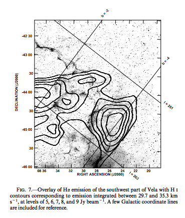
  • ​Radio: Radio emission is one of the best regimes to identify supernova remnants and classify them. Radio emission is often coupled to the X-ray radiation present and can give information on the electrons responsible for emission in both wavelengths. Radio waves can also map the supernova remnants’ surroundings, showing what pre-existing neutral matter might be lurking in the vicinity of nearby shockwaves. 
  • ​Infrared (IR)​: IR emission can show dust from the surroundings that has been swept up by the supernova remnant shock wave and has been shocked and heated.
  • Optical: Filaments visible in the optical regime can tell you how the shock wave has impacted pre-existing clouds of material. Filaments form when the ambient material is shocked and heated. A really good indicator of a shock-cloud interaction is confirming an optical filament that coincides with a bright X-ray boundary. This is supportive that you have found the position of the shock wave boundary of the remnant and its surroundings, indicating it is pushing up against something.
  • X-ray: This regime alone tells you a lot about the morphology of a supernova remnant and potentially even what type of explosion occurred that gave rise to this emission.  X-rays do a great job of showing you where the shockwave is in space because the material that is swept up, shocked, and heated, will be excited enough to radiate a lot in this regime. Finding those boundaries and comparing across wavelengths can make a more complete picture. 
  • Gamma-ray: Gamma-rays tell you an environment has been disturbed so aggressively, the particles are accelerated to very high energies. Gamma-rays are also the product of cosmic rays interacting with ambient material. Because cosmic rays are observed to be mostly protons or ions, we look for gamma-ray signatures that indicate a high proton population presence and acceleration mechanism.

Tying all of the information from each wavelength together creates a robust picture in order to determine if a shock-cloud is in fact happening. When gamma-ray emission is present as well, this presents the possibility for particles to be efficiently accelerated at the shock-cloud boundary to cosmic ray (CR) energies that then decay to gamma-rays when interacting with their dense surroundings. 

What we want to do next then is understand more about the shock-cloud boundary we have discovered to the west of the Vela SNR. We performed broadband modeling to try to see if we could constrain the gamma-ray models using either 1) leptonic gamma-ray emission (i.e. electrons via nonthermal bremsstrahlung or inverse Compton scattering) or 2) hadronic gamma-ray emission (i.e. proton-proton collisions generating the observed emission) but this is really hard to do, as both particles generate very similar gamma-ray signatures. Unless you have lots of data to confirm if the pion bump can be best fit to the data, it can be hard to rule out either scenario. The pion bump is the gamma-ray signature we look for for hadronic gamma-ray emission. I’ll show you what I mean.

The pion bump is the result of CR protons’ interaction with other ambient, less energetic protons. The protons collide and decay to neutral pions which then decay into gamma-rays. The gamma-ray signature will show up at the rest mass of the decayed neutral pion. On a standard spectral energy distribution (SED) plot, that would be around 200MeV. Here is a really great article discussing observations and modeling looking for the pion bump.

Above is the gamma-ray spectrum of the supernova remnant as measured with the Fermi-LAT and AGILE. Purple-blue shaded areas bound by dashed lines show the best-fit broadband model (60 MeV to 2 GeV) and the gray-shaded bands show systematic errors below 2 GeV due mainly to imperfect modeling of the galactic diffuse emission (i.e. background). There is a lot here. Let’s unpack it together.

The first line indicated is showing you the best fit model for the gamma-ray emission, regardless of the particle population, and only dependent on the energy distribution. The data points are taken from two different telescopes 1) Fermi and 2) AGILE, another gamma-ray telescope. The solid purple-blue line models the emission if it were from pion decay (i.e. the pion bump). The dashed purple-blue line corresponds to the electron population generating the observed emission via nonthermal Bremsstrahlung. The dash-dotted line is a modified electron population generating the observed emission via nonthermal Bremsstrahlung. A careful inspection of this plot shows that the data points follow the pion decay model the best, thus confirming that the gamma-ray emission for this supernova remnant is dominated by proton-proton collisions, and hence makes W44 another candidate for fresh CR acceleration. This means the environment is energetic enough to produce their own CRs, as opposed to just boosting up pre-existing CRs that get tangled in the region.

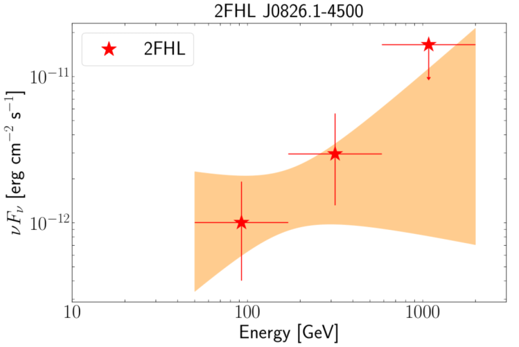
With our SED, things are not so clear. It is shown below and is also discussed in the paper.

The arrows indicate upper limits. This means the data could fall anywhere under the upper limit data points. Therefore, we see, within the uncertainties of all our data for the Vela shock-cloud boundary, anything is possible! So we are not able to gain any insight to the likelihood of fresh CR acceleration occurring here based on SED modeling alone, unfortunately. Note: in both of these images, try to bog down that pion bump at 200MeV. It’s easier to see on our plot since we plot the energy already in MeV. The three solid curves modeling the gamma-ray emission, they all steeply rise beginning at about 200MeV – that’s the pion bump!! 

But it is not a lost cause. There are other things to look for. This requires a deeper investigation into the properties of the shock itself. If we can determine the interaction is relatively new we might be able to say fresh CRs are produced here. However, if the shock has pushed into this cloud for a while, it has probably lost a lot of speed with respect to the rest of the shockwave and thus, loses more opportunity to accelerate particles to CR energies. Ways we can do this are by looking back in the optical and looking for tracers that tell us if the shock has gone radiative.

When a shock has gone radiative, this is when rapid cooling takes place and will dominate with time, sucking energy away from the shock and dispensing it into its surroundings. When rapid cooling starts, elements can “recombine” and will radiate via optical radiation, further instigating the cooling mechanism. The first elements to show up are oxygen, silicon, and nitrogen. Specifically, O [III], Si [II], and N [II]. These are ions of the elements, where the numbers indicate the loss of electrons. For example, oxygen should have 8 electrons (just by looking at the periodic table), but its doubly ionized in O III, which means it only has 6 electrons (and therefore has a positive charge of 2+ because it now has 2 more protons than there are electrons). Therefore, observing the shock location in the optical range where these ions radiate when present will tell us if the shock is radiative, and whether it can freshly produce cosmic rays by itself in the shock-cloud boundary.

So we ask for time on an optical telescope, the Gemini telescope in Chile. It is an 8-meter telescope with spectacular angular resolution so we can probe the shock with sub-arcminute resolution to find radiative tracers. We ask for both imaging and spectroscopy to do a thorough study in this band. We got both! In my next post on this, I will share with you the preliminary findings from the imaging, which are spectacular to look at. Optical astronomers are so lucky – they produce such beautiful, whimsical, and informative images. The spectroscopy, on the other hand, is amazingly hard to reduce. Currently, I have no results from the spectroscopy (that make sense). This should excite you as I have yet to publish any results on these optical images but yet, you will be able to see them here first! 🙂

• Gamma-ray emission uncovered to the west of the Vela SNR
• Investigations of this region in the X-ray uncover soft, diffuse X-ray emission overlapping with the gamma-ray position
• We now look across the light spectrum using Aladin (free for everyone and you don’t need to download anything. It’s truly amazing – See over a dozen sky maps across the light spectrum right now: https://aladin.u-strasbg.fr/AladinLite/)

​Click the link above. I’ll show you how we found our optical counterpart. Type in “08 26 07 -45 00 00” verbatim, double check you have “DSS2” selected. Hit ENTER. Do you see a thin film of material move downwards from the crosshair in the center of the screen? Yeah – that’s our optical counterpart and you just found it using the gamma-ray emission’s coordinates.

Now the real fun sets in: I begin digging. Digging for information about the Vela SNR. How old is it? i.e. When did the progenitor star explode? What type of supernova was it? How far away is it? What available information is known, specifically coinciding with this gamma-ray emission?

Here’s what I found out. 

Vela is about 10,000 years old descending from a Type II supernova which we have discussed before here. Because it is a type II supernova remnant, it houses a pulsar, the remnant of the star’s explosion which powers a pulsar wind nebula that is quite large. Vela as it turns out is the closest composite SNR to Earth which means there are tons of literature about the region. I read dozens of papers studying Vela from the radio to the gamma-ray. It became apparent that the pulsar wind nebula is huge and is seen brightly in all wavelengths and so is the pulsar. The remnant itself was only known to generate gamma-rays 1.2 degrees away from the pulsar or about 15 parseconds (50 light years) but in the opposite direction of where we found the new gamma-ray emission and we are still not really sure where the gamma-rays in this other region come from. It’s possible it could be another interaction site (which I’ll get to).

Because Vela is a Type II supernova remnant, this means the area surrounding the remnant is quite dense compared to other regions of space. As a refresher, let’s remind ourselves that Type II supernovae occur when a seriously massive star explodes. Massive stars have shorter lifespans than smaller stars because the larger the star is, the faster it burns its fuel. Once it runs out, it explodes. The largest stars have lives as short as a few million years old. For comparison, our star, the Sun, is very “average” in size and will not explode at end of life but will rather complete a few evolutionary stages before shedding it’s layers and retiring to the white dwarf stage – which will take our Sun a total of 10 billion years. So, when a massive star is born, it is born into a dense environment of stellar gas, a stellar nursery, if you will. The most massive stars die off and explode the quickest and thus never leave the dense region of stellar gasses, so when it explodes, the explosion is typically very asymmetrical and quite complicated due to the complexity of the region. As the initial blast wave plows into interstellar space, it will readily interact with material already here like gas, dust, molecular clouds and clumps, etc. Depending on how fast the initial blast wave is and how dense the material is, it interacts differently. If the shock wave is still hugely fast, it will sweep up this material, shock it, and move it with the blast wave itself. If it is has slowed down considerably, it will run into the material and slowly shock and heat it as the shock wave dissipates into​ the material. The timescales of these interactions depend on the density of the material. 

Why am I talking so much about a remnant’s surroundings? Oh right, so, Vela is a Type II SNR which means that its surroundings are probably pretty clumpy. In fact, in 1998, when I was 4 years old, radio astronomers pointed their telescopes at Vela and saw an abundance of neutral hydrogen out here. They came to the conclusion that these structures were pre-Vela, or pre-existing. What likely happened is another massive star, possibly millions of years ago or more, exploded and its SNR expanded to be this entire huge neutral hydrogen bubble expanding into deep space and by the time Vela came along, the medium was made up of dense, clumpy clouds from the leftover material of this long-ago supernova, leaving plenty of opportunity for a fresher remnant to interact with it. 

This was the same paper I noticed our optical counterpart was being studied. Like, our exact optical filament, believed to be associated in some way to the mysterious gamma-ray emission, was being discussed and implicated in a theory in this paper, that was published over 20 years ago. 

I remember it vividly – figure 7 of her paper – showing me that our instincts were, in fact, right. We suspected the blast wave of the remnant to be running into something, generating the emission we were observing. This 1998 paper confirmed what we thought and provided the last piece of the puzzle: the something it was running into. A small neutral hydrogen cloud, at the same position of the optical filament. What’s more is that they shared not only the same region of space, but also opposite curvature. You can see it in the picture above. See how the filament seems to trace the contours of the hydrogen cloud? Finding “puzzle pieces” like this is actually pretty substantial evidence that these two are not only connected, but are telling you an interaction between some type of shock wave and a cloud is occurring. 

​We found older X-ray maps from a previous mission, ROSAT (The Roentgen satellite, named after the scientist who discovered X-rays), that mapped the entire Vela region in the soft X-rays. You can see in the image, appended below, where our source lies with respect to the entire remnant. Let’s spend a few minutes dissecting the image for a more wholesome understanding, then we will loop back to the important piece of evidence here.

We see the entire remnant right – looks almost fully spherical in the X-rays. Compared with Vela in the optical here, it looks quite different, doesn’t it? In the X-rays, it’s nature is obvious. This emission is found to be mostly from really hot particles from the blast wave and from stellar ejecta that have been swept up as the supernova expanded into its surroundings. You can identify a few “break out” regions, one is directly to the left (east) and the other is more subtle, and fainter, directly to the west (right) and much farther out. These break out regions are indicators for how the density in the interstellar medium changes. Where the blast wave has been able to break into indicates less dense regions. Where the bright boundaries exist, this indicates where the blast wave has coincided with denser material, shocking and heating it as it begins to slow down due to the blockage.

So, essentially the bright X-ray boundaries give you a little information about the 1) density of the surrounding medium and 2) speed of the shock there and 3) where the remnant ends and the surroundings begin.
​
In summary, we have an optical filament attached to both the X- and gamma-ray emission to the west, that is now also associated with a neutral hydrogen cloud and they share opposite curvature, and all of this coincides with a bright X-ray boundary. 

…. What? You thought this is where the story ends? Heck no! This is just the beginning. Now that we have established that the SNR is interacting with its surroundings – we just confirmed the Vela SNR as a candidate for fresh cosmic ray acceleration.

Recall that SNRs and PWNe are some of the most extreme objects in our galaxy and are thought to generate the bulk of Galactic cosmic rays. So a new challenge has revealed itself to us: Can we establish the Vela SNR and its shock-cloud interaction as a possible site where cosmic rays are produced?

Ah, right. The new gamma-ray emission on the west of the Vela supernova remnant. After retrieving all of the known data available to us about this region, we started to piece together the puzzle. Here’s what we know!

1. New gamma-ray emission is uncovered directly to the West of the Vela SNR.
2. The gamma-ray emission is very high in energy, that is, all of the energy is detected above 50GeV.

But that’s it. We don’t know why gamma-rays are emitting at this one small section of the remnant. We don’t know what event occurred for this to happen. We don’t know what particles are responsible for the emission. Instead, we used this information and what it implies to make the next step: submit a proposal to view the region in X-rays. X-rays are also pretty high in energy but what makes this wavelength regime appealing to us is that present telescopes that can image in the X-ray have spectacular angular resolution compared to gamma-ray telescopes right now, i.e. we can see more features and distinguish between sources easier in the X-ray than in the gamma-ray. For example, the XMM-Newton X-ray space telescope  has an angular resolution on the order or arcseconds. This is 1/3600 of one degree. In comparison, a full moon is roughly 1/2 a degree in our sky so 1 arcsecond of the moon would be 1.388×10^(-4) (or 1/7200) of the Moon we see which is a really tiny, tiny, tiny part of the moon. We would not be able to resolve 1 arcsecond with our own eyes. Nor would we be able to resolve 1 arcminute (which is 1/60 of a degree or 1/120 of the full Moon) with our own eyes. The Fermi-LAT, on the other hand, can resolve very high energy (VHE) sources on the order of arcminutes. So, the angular resolution in the X-ray regime is much more attractive in our endeavor to try to find more information about this new gamma-ray source. 

Furthermore, the X-ray sky is somewhat less crowded. The gamma-ray sky has a lot of diffuse, or spread out, emission across the sky. A lot of this comes from our Galaxy as well as extragalactic sources (sources that are not in this Galaxy) and this can be especially distracting near the Galactic plane (see image below). We now know that the entire gamma-ray sky is full of gamma-ray emission coming from all over the Universe! The X-ray sky also has a diffuse background but it is a little easier to work with. 

So for this reason, we asked for time on the XMM-Newton X-ray space telescope to observe our peculiar source and we got it! After cleaning the data we received from the telescope, we were able to study the X-ray emission that exists at the same location in space as the gamma-ray emission we see. We indeed found an X-ray counterpart which is a compelling overlap in both shape and position for the X-ray and gamma-ray emission. The other nice thing about looking in other wavelengths, if you can find one positive counterpart, you can then use this new information to look further into other wavelengths to see what other emission this region might be giving off. That’s exactly what we did! The images below reveal the X-ray emission we see after cleaning up the data and the first counterpart we found by using the position of our gamma- and X-ray data and the shape we resolved with XMM-Newton​.

A picture is starting to form in our minds… We have gamma-ray emission that is very concentrated to the west of the Vela supernova remnant that has soft, or low-energy, X-rays tracing out an optical boundary or filament. Something must be happening at the edge of the remnant here for it to be so energetic with so many puzzle pieces. We started leaning towards the idea that maybe the remnant is running into something here and is shocking it. Imagine a hot, really fast-moving wave of heavy mass hitting a cold, slow clump of gas. A lot of mixture, turbulence, and violent disruption happens on many scales. You would expect the cold, slow clump of gas to ignite in some way; the gas particles responding rapidly and enthusiastically with its new momentum from the collision, colliding into each other and gaining massive amounts of energy at the collision boundary. It begins to illuminate its surroundings as these interactions take place, heating the gas and shocking it further. The gas clump likely feels an incredible increase in its temperature. 

It seems reasonable then that this is in fact what we are seeing but we cannot say for sure. If this work will be worthy to publish, we need concrete evidence that a shock-cloud interaction is taking place and causing the emission we see. So, we keep digging for more puzzle pieces.

Cosmic rays are a wild phenomenon. They are relativistic electrons, protons, and other heavier nuclei that are traveling almost at the speed of light. About 90% of all cosmic rays are known to be protons while the rest make up the other 10%. It’s amazing to see these massive particles moving so close to the speed of light because it means they must have come from an immensely violent origin for the particles to have attained such high energy. It’s important to note that cosmic rays are distinct from light in that light particles are completely massless and neutral in charge (i.e. they do not have a charge).  We know these particles exist – they bombard Earth from all directions and from a variety of sources, one including our Sun. High energy astrophysicists want to know what sources are capable of producing such high energy particles.

However, this question is not a straight forward one to answer. These particles not only have a mass but, they also have a charge. A charged particle readily interacts with magnetic fields which is a prominent feature throughout the Galaxy and the objects it contains. This makes tracing a cosmic ray’s path back to its origin, like we are able to do with light particles, incredibly difficult. The image below (right panel) illustrates a complicated cosmic ray path, rendering it impossible to know where in the Galaxy this cosmic ray formed. The left image shows us real data measured from Earth, showing us the spectrum of cosmic rays we have detected. Don’t freak out – a spectrum is simply a graph that shows you which energy range contributes the most to the flux we observe. The flux you may think of as the emitted power of the object as observed from Earth. For example, we see the lowest energy cosmic rays contribute the most to the overall flux by studying the observed spectrum (displayed in the left image below) because the peak of the spectral flux (on the y-axis) occurs at the lowest energies (x-axis). Additionally, right around the 10^6GeV (or 10^15eV) mark on the x-axis roughly tells us where Galactic cosmic rays cap off; cosmic rays with greater energy than 10^15eV must be explained by something even more energetic than any object known in our Galaxy. We therefore identify cosmic rays with energy less than or equal to 10^15eV Galactic cosmic rays and cosmic rays with energy greater than 10^15eV extragalactic cosmic rays. ​

Now that we have a good grasp on what cosmic rays are and why we are so interested in them, I present to you the first source I extensively studied. It started out as an unidentified gamma-ray source discovered by Fermi at very high energies. We’re talking about energies above 50GeV which is on the more energetic side of the gamma-ray energy range.

The unidentified gamma-ray source led to my first published paper and was the basis of my Master’s thesis. I will link both at the end of this blog post!

In addition to a new, very high energy, gamma-ray source being discovered, this unusual guy also has some interesting characteristics. It’s spectrum in the high energy range (above 50GeV) is what we describe as hard. This means the majority of the flux is dominated at seriously high energies and increases rapidly with energy. We can describe its spectrum in this range with a power law. A power law models the observed flux assuming the energy falls off with a given power law index. For example, gravity behaves like a power law – its strength decreases with increasing radius with a power law index of 2. The smaller the power law index, the more dramatic this behavior would become. So in the gamma-ray energy range, when we see a very hard spectrum with a small photon index, this indicates there is efficient particle acceleration occurring here – i.e. the environment generating these gamma-rays is also probably accelerating massive particles close to the speed of light. This further implies that this environment could be generating its own cosmic rays and injecting them into the Galaxy. This was intriguing to discover so the first thing we did was see where in the sky it is located. We look at the objects around it, determining if this is truly a newly discovered candidate accelerator or if a known source in this region of space is now being detected at such high energies. I should mention that the special thing about this source is that it was reported in a catalog of objects using the Fermi-LAT with a brand new software update that enabled the instrument, for the very first time, to detect gamma-rays at energies above 50GeV. The official name of this source is 2FHL J0826.1-4500 which you see in the images below. For the purposes of this blog post, I will name it “Geronimo“. 

2FHL in the name stands for the second (2) Fermi-LAT High Energy Catalog. The numbers following represent its equatorial coordinates (in J2000). In other words, any astronomer anywhere in the world can find where this source is located in the sky using its Right Ascension (R.A.) of 08:26:07 and declination (Dec.) of -45:00:00. Almost all astronomical objects are given official names based on their coordinates in the sky. You will typically see either equatorial or Galactic coordinates used. 

You see in the image to the right above that the source lies exactly west of the Vela complex which is a composite SNR. The Vela SNR is the closest composite SNR to Earth at only 290 parseconds or almost 1,000 light years (or 5.879×10^15 miles). This might sound incredibly far to you but in the grand scheme of things, the Sun and the Vela SNR are almost right on top of each other when you look at where they lie with respect to the rest of the Galaxy. I have a really cool schematic from a published article that I’ll try to find to illustrate this! 

When we saw how close in the sky this unfamiliar gamma-ray source was to the Vela complex, we began to dig deeper into the Vela region to try to understand the possibility of this source being associated to Vela in some way. This required a thorough multi-wavelength analysis. This entailed grabbing all information known about Vela in all wavelengths of light: radio, microwave, infrared, visible, ultraviolet, gamma-ray, you name it. I tracked all published work on the Vela region and read it. What we found is that this source is indeed a by-product coming from an interaction of the Vela SNR moving into its surroundings. Before we go any further, how about a quiz to make sure we’re all on the same page? Then, we can move onto Part II: how the different wavelength information helped us piece together what is happening to the west of the Vela remnant! 

I’m assuming you have already read the first blog post and will use the terminology we have established there. If you haven’t read it yet, click here!

What are composite supernova remnants?

Now, stars evolve based on how much hydrogen they have to burn. The more hydrogen you have, the more you burn, the faster you reach the white dwarf stage. Kapeesh?

Take one massive stellar companion and pair it up with one comparable in size, but smaller. Such that the more massive star will reach the white dwarf stage first. In this scenario, you have a white dwarf evolving around a middle-aged star that begins to enter its red giant phase. That means the white dwarf star is orbiting a star that is beginning to expand significantly into the orbit of the white dwarf. If the two stars are close enough, the white dwarf can actually start capturing matter from the surface of the red giant! We call this accretion. A white dwarf can accrete matter from its stellar companion if they are close enough in space. This causes a problem though. The white dwarf is already SO HEAVY. IT’S SO DENSE. IF IT TAKES ON TOO MUCH MASS IT WILL LITERALLY EXPLODE.

What is left behind after a Type Ia supernova explosion?
Answer: Nothing. The white dwarf explodes so violently, it obliterates the entire stellar system, leaving behind no core, no pulsar, nothing but the ejected mass that has been sent hurling through space at monstrous speeds. I guess I’m lying to you a little though because it’s not nothing. What is left behind is a bright and energetic supernova remnant left to its own demise as its mingles with the interstellar medium (i.e. the space and gas and dust that exists between star A and star B).

But, I still haven’t even touched on CC supernova remnants which is a great segue into composite supernova remnants, as composite remnants describe many CC supernovae. But since we already know what causes a Type Ia supernova, it’ll be easy to describe:
Take one really massive star that is at least 8 times the mass of the Sun. When the star runs out of hydrogen to burn in its red giant phase, the only thing left keeping the star from collapsing in on itself is the electron degeneracy pressure (oh, fancy talk!). The star is too massive at this stage to withhold the outer layers of the star against the iron core so, what happens? Kaboom!! A CC supernova occurs. This time what is left behind is a supernova remnant and the remaining core of the progenitor star (more fancy talk!). The core of the progenitor star is the neutron star and often powers a pulsar wind nebula. 

And just like that, we are familiar with the two most common types of supernova remnants found in our Galaxy. CC supernova remnants are the remnants that can be considered composite.

A composite supernova remnant is one that has all three components from a CC supernova: a pulsar, a pulsar wind nebula, and a SNR shell. All of these things have signatures in the light they give off and can be identified this way. ​

Let’s briefly discuss the other two types of remnants and how we can distinguish between them all!

Shell remnants: Observed emission from these systems is dominated by only the shell of the remnant. Remnants of either class could be categorized as such (i.e. Type Ia or CC). A ring like structure that often radiates in radio and X-ray wavelengths is commonly seen with shell remnants.

Crab-like or plerionic remnants: Aptly named after the famous Crab nebula, Crab-like or plerionic remnants are CC supernova remnants that have observed emission coming mainly from the pulsar and/or pulsar wind nebula. The emission that comes from the pulsar and pulsar wind nebula is mostly attributed to highly relativistic electrons and positrons. 

It is sometimes observed for an SNR to have a filled center as opposed to a ring like structure. Depending on the nature of the emission, it could be thermal X-rays from hot supernova ejecta or non-thermal emission from the pulsar wind nebula.

In general, emission from the shell of the SNR can be thermal or non-thermal in nature; thermal emission can be radiated by hot gas that is along the edge of the SNR’s front shock and being close to thermal equilibrium, i.e, all of the particles here emit radiation at the same temperature. If the plasma is not in thermal equilibrium, then it is non-thermal in origin. We often see non-thermal emission from the plerion. In both instances, we can model with good precision the temperature (for thermal) and the behavior of the particles and thus understand where the emission (whether it’s X-ray or else) is coming from. A composite supernova remnant has emission from both the shell and the plerion.

Finally, in summary, we can also identify Type Ia and CC SNe based on the elements present in their spectrum. This is a very basic rule but it is a good one for Type Ia and Type II supernovae (note: CC supernovae are a type of Type II supernovae. For now just know that – we can revisit other types of Type II SNe later):
If you see hydrogen emission lines in the light spectrum of the SNR, it is likely a Type II supernova remnant. If you do not see hydrogen emission lines in the light spectrum of the SNR, it is likely a Type Ia supernova remnant. I use the word “likely” because its probable based on this rule but, there are other indicators! For example, the location of the SNR, the density of the surrounding region, and other emission lines in their spectra can provide clues to the event that occurred for the SNR to exist.

For more information I love using this website for educational outreach: https://imagine.gsfc.nasa.gov/science/objects/supernova_remnants.html. There are other great resources listed at the end of the article as well. ​